Algorithm Description
Introduction
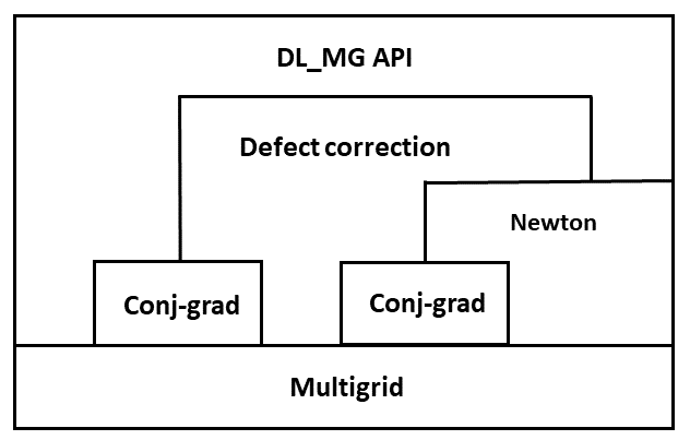
The above diagram show the main ierative layers of the solver and the posible combination in which the solver can be used.
Multigrid Layer
The main components of the mutigrid solver used in DL_MG were selected following the standard recommendations for PE and PBE solvers. The grid stencils are derived by discretisation of the differential operator at each level (geometric approach) with the finite differences method using 7 point stencil. Coarsening is achieved by doubling the lattice constant in all dimensions, smoothing uses Gauss-Seidel red-black method, inter-grid transfers are performed with half-weight restriction and bilinear interpolation. With these components one can build a close to optimal and efficient solver for the PE and PBE, provided that the models used for the permittivity and charge density are smooth and without strong anisotropies Trottenberg.
The V-cycle was selected for multigrid iterations as generally recommended for parallel computations Trottenberg, Chow. MPI parallelism is used for data decomposition; the cuboid global grid can be distributed amongst MPI ranks using general 3D,2D or 1D topologies. As the coarse grids are derived from the fine grids by removing the points with even index coordinates in all directions, no data is exchanged between MPI ranks during inter-grid transfers. The number of MPI ranks can vary across multigrid levels because some ranks could be assigned zero grid points below a certain coarsening level, depending upon the global grid size and MPI topology at the finest level. MPI communication at each level is done in a separate communicator that includes only the active ranks. Domain halos are exchanged with non-blocking sends and receives, the edge and corner points of the local domains are transfered between ranks by using ordered communication along axes between nearest neighbours Trottenberg.
Conjugate Gradient Layer
The standard preconditioned conjugate gradient is implemented in dl_mg_conjugate_gradient_method:: . Experiments done with ONETEP and some simple charge distributions tests have shown that conjugate gradient with multigrid preconditioner is useful when the multigrid solver struggles to converge or the number of multigrid level is less than about 4. When the multgrid has a fast convergence the conjugate gradient degrades the solver performance (about 10% but with large variation from case to case).
The conjugate gradient solver is not enable by default in the current version. If enabled (via the interface argument or by setting the environment variable DL_MG_USE_CG=T) the multigrid preconditioner uses one V cycle by default.
Newton Layer
The non-linear solver algorithm is impelmeted in dl_mg_newton_method:: and it follows closely Holst paper.
Defect correction layer
The higher order discretisation correction for the space derivatives can be added to the second order solution obtained with the multigrid or Newton solvers. The finite difference approximation for the potential derivatives can be computed for orders \(k=2p,\ p=2,\dots,6\). Asymmetric formulas are used at the boundaries in the case of Dirichlet boundary conditions.
The correction is computed iteratively starting form the expression
\[ A_k(\phi_2 +\delta_k) = f \]
where \(A_k\) is the lhs of PE or PBE which uses finite differences of order \(k\) for the derivatives, \(\phi_2\) is the second order solution obtained with the multigrid or Newton solvers, \(\delta_k\) is the higher order correction and \( f\) is the charge density. An approximate higher order correction can be computed efficiently by using the second order operator as an approximation for \( A_k \), that is
\[ A_2 \delta_{k}^{(n+1)} = f - A_k \phi_{2}^{(n)} \ .\]
The found \( \delta_{k}^{(n+1)} \) is added to the current potential and the procedure is repeated until the convegence test is satified. In the case of PBE \(A_2\) in the above equation is the linerisation of the PBE operator around the current value of the potential.
An error damping procedure is provided that can be used to find a scale factor \(s\) for the correction \( \delta_{k}^{(n+1)} \) such that the defect norm decreases during iterative process, i.e.
\[ || A_k(\phi^{(n)} + s \delta^{(n+1)}) -f || < || A_k(\phi^{(n)}) -f || \]
with \(s \le 1\). This can help to find the solution for cases which don't converge or have a poor convergence rate.
Permittivity discretisation
The solver needs the values of the relative permittivity \( \epsilon (\vec r) \) at the grid points and also at the points half way between the next neighbors grid points. This is so because the second order finite difference discretisation uses a centered scheme
\[ \partial_x[\epsilon(\vec r_i)\partial_x\phi(\vec r_i)] \rightarrow [\epsilon_{i+1/2}\partial_x\phi(\vec r_{i+1/2})- \epsilon_{i-1/2}\partial_x\phi(\vec r_{i-1/2})]/h \rightarrow \\ \frac{\epsilon_{i+1/2}\phi_{i+1} - (\epsilon_{1+1/2}+\epsilon_{i-1/2})\phi_i+\epsilon_{i-1/2}\phi_{i-1}}{h^2}, \]
while the higher order finite differences scheme use the expanded version of the differential operator
\[ \nabla[\epsilon(\vec r)\nabla\phi(\vec r)] = \epsilon(\vec r)\Delta\phi(\vec r) + \nabla\epsilon(\vec r)\cdot\nabla\phi(\vec r) \]
which is discretised only with grid point values. The midway values of the relative permittivity can be provided by the calling application in the solver argument eps_mid or they can be computed by the DL_MG as the harmonic average of the neighboring grid values, see compute_eps_half_loc(). In order to use the internally computed midpoint values the application has to set eps_mid= dl_mg_eps_mid_ignore in the solver call.
Tests done with the harmonic average approximation have shown acceptable deviation from the solution computed with the exact midway value of the relative permittivity even in the case of fast varying function. However, a subset of test cases in ONETEP have produced large deviations when this approximation was used.
Note: eps_mid can be used for problems in an anisotropic medium with a diagonal permittivity tensor, but only with the second order finite differences scheme.
Parallelism details
OpenMP parallelism is implemented using one parallel region that covers the V-cycle loop. All other loops from higher levels over the computational grid are also parallelised. The local MPI rank domain is decomposed in thread blocks with an algorithm that searches for optimal work partition, see dl_mg_omp:: . MPI communication inside OpenMP regions is handled by the master thread (the so-called funneled mode), mainly for reasons of portability. Data transfers between MPI buffers and halos are done using one thread per local grid side with the help of single directives.
More details on implementation and performance are available in JC Womak 2018 and these reports: 1, 2.
Convergence Criteria
DL_MG uses the following convergence test for the multigrid and Newton solvers
\[|| r || < \mbox{max} (\tau_{\mbox{abs}},\, \tau_{\mbox{rel}} || \alpha \rho ||) \ ,\]
where \( r \) is the corresponding residual. For the higher order discretisation correction the convergence is achieved at step \( i+1 \) if both following conditions are true:
\begin{eqnarray*} ||\phi^{(i)} -\phi^{(i+1)}|| & < & \mbox{max}(\tau_{\mbox{abs}}^{\phi},\, \tau_{\mbox{rel}}^{\phi}||\phi^{(i)}||) \\\ ||r_{k}^{(i+1)}|| & < & \mbox{max}(\tau_{\mbox{abs}}^{r},\, \tau_{\mbox{rel}}^{r} ||r_{k}^{(0)}||) \ , \end{eqnarray*}
where \( r_{k}^{(i)} \) are residuals of the higher order correction iterations. In both cases the set of parameters \(\tau_{<>}^{<>}\) are chosen with sensible default values and they can be set via optional arguments, see dl_mg::dl_mg_solver_poisson(), dl_mg::dl_mg_solver_pbe().
If the PBE solver is run with the constrain to conserve the number of ions for the electrolyte, see Periodic boundary conditions (PBC) for PBE, an aditional convergence test for the excess chemical potential \(\mu_i\) is used:
\[ | \mu_i^{(i+1)}-\mu_i^{(i)} | < \mbox{max}(\tau_{\mbox{abs}}^{\mu},\, \tau_{\mbox{rel}}^{\mu}|\mu_i^{(i)}|) \]
in Newton and defect correction loops.
The solver has default tolerances set for all iterative layers. The user should try to set the convergence parameters for the top layer with the solver arguments tol_res_abs and tol_res_rel. For hard to converge problem changes of the convergence tolerances and/or the number of maximum iterations in the lower iterative layers might be useful.
Note: In the case of the second order finite difference there is an ambiguity if both, a generic argument tol_res* and a specific argument (i.e. tol_cg_res*) are present in call argument list. The convention used is that the specific argument supersedes the generic argument. If the finite difference order is larger than 2 then the generic convergence argument applies only to the defect correction layer.
Periodic boundary conditions (PBC) for PBE
In the case of PBC the Laplacian operator cancels the potential zero mode on the lhs of PE or PBE equations therefore for consistency the charge distribution on rhs has to satisfy the same condition, i.e.:
\[ \int_V \left[\alpha\rho(\vec r) + \lambda\sum_i q_i c_i \gamma(\vec r) \exp \left( -q_i\beta\phi(\vec r) \right) \right]dv = 0 \]
where \( \gamma(\vec r) = \exp (-\beta V (\vec r)) \) is the steric weight function.
DL_MG ofers several option to satisfy the neutrality condition:
Uniform background (jellium) neutralisation
One way to satisfy the charge neutrality constraint is to neutralise the solute charge with an uniform background of opposite charge whose density is chosen such that the total charge in the computation cell is zero, i.e., \( \rho(\vec r) \rightarrow \rho(\vec r) -(1/V)\int_V\rho(\vec r)dv \). It follows that the total charge of the electrolyte is zero and one has to fix the chemical potential of each electrolyte species such that average concentration in the computational cell is the bulk concentration J Dziedzic 2020. In some more detail we have as follow: Starting from a mean field free energy functional one can show that the ions concentration depend on the excess chemical potential introduced by the steric potential \(\mu_i^{ex}\) and on the electrostatic potential contribution to the chemical potential \(\mu_i^{el}\):
\[ \mu_i = \mu_i^{ex} +\mu_i^{el} = -\beta^{-1}\ln\Gamma +\mu_i^{el} \]
where \(\Gamma = (1/V)\int_V \gamma(\vec r)dv\) is the fraction of accessible volume for ions.
With these definitions the concentration of species \( i \) can be rewritten as follows:
\[ c_i^{PBC}(\vec r) = \frac{c_i}{\Gamma} \gamma(\vec r)\exp \left (-\beta q_i\phi(\vec r) + \beta\mu_i^{el} \right) \ . \]
From the ion number conservation condition \(N_i = c_i V = \int_V c_i^{PBC}(\vec r) dv\) one can derive the following equations for the excess electrostatic chemical potentials:
\[ \mu_i^{el} = -\beta^{-1}\ln \left[\frac{1}{V\Gamma}\int_V \gamma(\vec r)\exp \left(-\beta q_i\phi(\vec r) \right) dv \right], \]
that must be satisfied together with PBE.
The ion concentration \(c_i^{PBC}\) is invariant under the combined shifts
\begin{eqnarray*} \phi(\vec r) &\rightarrow & \phi(\vec r) + \mbox{const} \\ \mu_i &\rightarrow & \mu_i + q_i\ \mbox{const} \end{eqnarray*}
The solver break this symmetry by selecting \(\phi(\vec r)\) with the property \( \int_V \gamma(\vec r) \phi(\vec r) dv = 0 \).
The above equations can be used to derive \( c_i^{PBC}(\vec r) \) for the linearised PBE. After a little algebra we find for the first order in \( \beta\phi \)
\[ c_i^{PBC}(\vec r) \approx \frac{c_i}{\Gamma}\gamma(\vec r)\left[1 - \beta q_i(\phi(\vec r) - \bar\phi)\right] \]
where the potential shift
\[ \bar{\phi} = \frac{1}{\Gamma V} \int_V \gamma(\vec r)\phi(\vec r) dv \]
ensures that the PBC condition is satisfied. As in the case on full PBE the solver returns \( \phi(\vec r) -\bar\phi\). For this choice it can be shown that \(\mu_i^{el}=0\) in the linear approximation. The linerised concentration is used to find the electrostatic potential by solving the linearised PBE. The ionic concentration should be compute with
\[ c^{PBC-\mbox{lin}}_i(\vec r) = \frac{c_i}{\Gamma} \gamma(\vec r)\exp \left (-\beta q_i\phi^{\mbox{lin}}(\vec r)\right) \]
in order the preserve the non-negative property of the ion concentration. The jellium neutralisation is the default selection in DL_MG when full PBC are used.
Neutralisation by electrolyte concentrations shift (NECS)
In many cases of interest PBC is an useful computational tool even when there is no natural background charge neutralisation for the solute. For these cases DL_MG can achieve electroneutrality by shifting the electrolyte concentrations from the bulk values such that the total charge of the computation cell is zero, i.e.
\[ c_i = c_i^\infty -x_i \frac{Q_s}{q_i V\Gamma} \ , \]
where \(x_i\) are the shift parameters and \( Q_s=\int_V \rho(\vec r)dv \) is the solute charge. The value of the shift of each ion species is found from the asymptotic condition on the electrolyte concentration ratios, see Bhandari2020. This method has several sub-cases which can be selected in the solver interface with of the parameters defined in this include file.
The solver interface returns optionally the values of the quantities used for neutralisation, such as chemical potentials \( \mu_i/(\beta T)\), steric weight average \( (1/V) \int_V e^{(-\beta V_{steric}(r))} dv\), shifted ion concentrations \( \{c_i\}\) , and concentration shifts \( \{x_i\}\).
A note on the definition of the ion concentrations: In the above expressions the average electrolyte concentrations are defined as \(N_i/V\) where \(V\) is volume of periodic cell. The previous expressions show that the average electrolyte concentrations defined against the ion accessible volume, i.e. \(c_i^{(\Gamma)} = N_i/(V\Gamma) = c_i/\Gamma\), is a more suitable quantity. Therefore the solver uses \(c_i^{(\Gamma)}\) and one should pay attention to use the correct definition for the corresponding argument of dl_mg::dl_mg_solver_pbe. This choice for the definition of average concentration is more suite for models in which the solute extends in the computational cell in one or two dimensions, e.g. a slab geometry.
Environment variables
Relevant parameters for the tuning of the iterative algorithm are provided as optional parameters in the API. However, in certain cases it might be useful to change these parameters without recompilation or changes to the input files. This can be with help fo the following environment variables:
| Name | values | Notes |
|---|---|---|
| DL_MG_USE_CG | T,t,F,f | enable/disable the conjugate gradient module |
| DL_MG_NITER_VCYC | integer | set the maximum number of V cycles for the multigrid solver |
| DL_MG_MAX_LVL | integer | set the number of multgrid leves to a lower value than the number of levels that generated by coarsening procedure |
| DL_MG_NITER_LEVEL1 | integer | maximum number of iterations to be done on the coarest level |
| DL_MG_V_ITER | "integer,integer" | number of relaxations to be done on the two branches of the V cycle |
| DL_MG_OMEGA_SOR | real | the parameter used for the succesive overrelaxation on the coarse multigid level |
| DL_MG_NEUTRALISE_NWT_START | real | sets the starting values for the computation of concentration shifts see Details of concentration shifts computation |
Grid Size Constrains
In order to generate enough multigrid levels, the global grid must have sizes given by \([q_1 2^{n_1}+\delta_1, q_2 2^{n_2}+\delta_2, q_3 2^{n_3}+\delta_3]\) with \(q_i \le 20\) for an efficient solution at the coarsest level. \(\delta_i\) is 1 or 0 for Dirichlet or periodic boundary conditions, respectively, in direction \( i\). Also, for a good multigrid convergence rate the ratio of the global domain sizes should not deviate too far form 1.